What is an ANN?
ANNs are computing systems inspired by the biological neural networks that constitute animal brains. ANNs are based on a collection of connected units or nodes called artificial neurons, which loosely model the neurons in a biological brain. You can see an example image of an artificial neuron below.
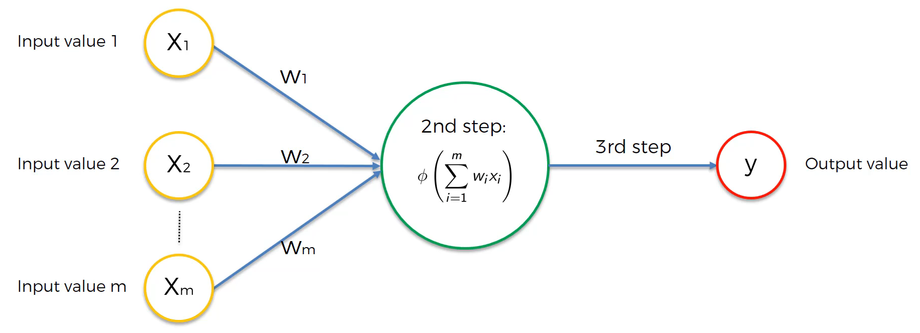
Each connection, like the synapses in a biological brain, can transmit a signal to other neurons. An artificial neuron receives signals, processes them, and can signal neurons connected to it. The “signal” at a connection is a real number, and the output of each neuron is computed by a non-linear function of the sum of its inputs.
How do Neural Networks Work?
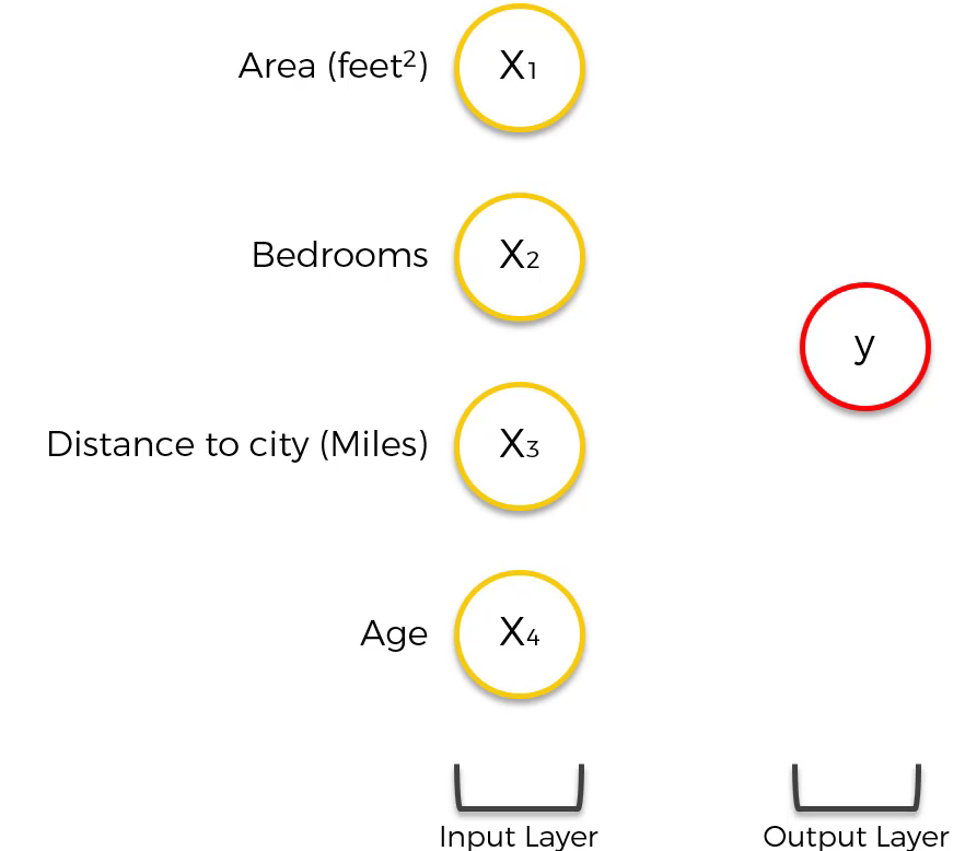
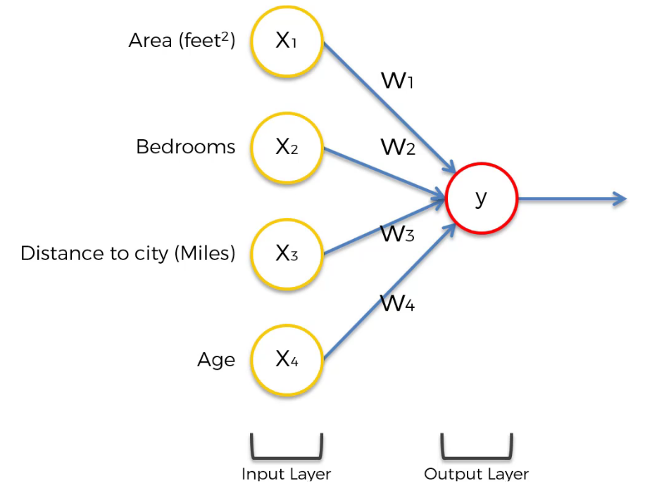
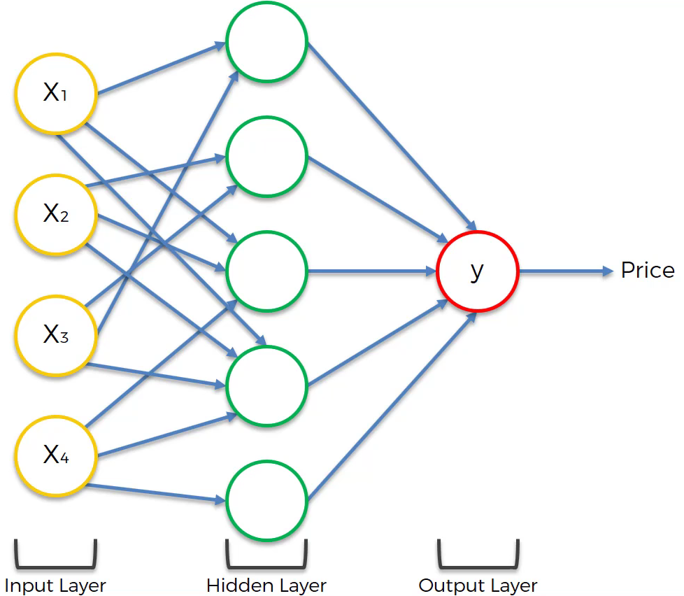
Assuming that we are predicting the price of a house and there are four input parameters (area, bedrooms, distance to the city, age). The basic form of a neural network has only an input layer and an output layer without a hidden layer, as shown below:
In this form, the input variables are weighted by the synapse, and the output layer is calculated by a certain algorithm. For example: $(\text{price} = w1 \times x1 + w2 \times x2 + w3 \times x3 + w4 \times x4)$
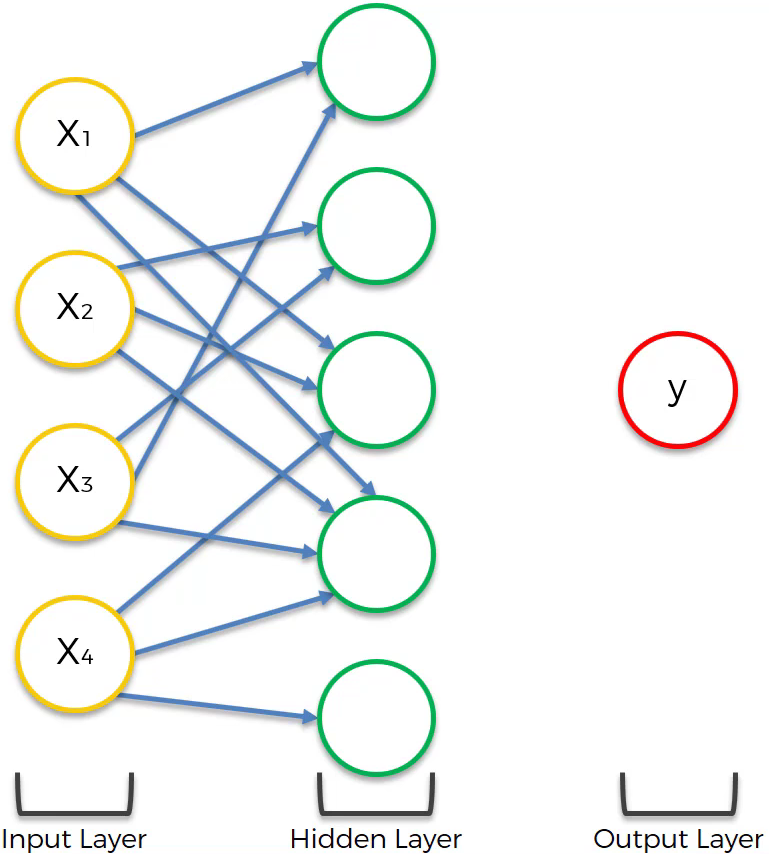
However, this form lacks the flexibility and functionality provided by ANNs. ANNs provide flexibility and functionality using hidden layers, as shown below:
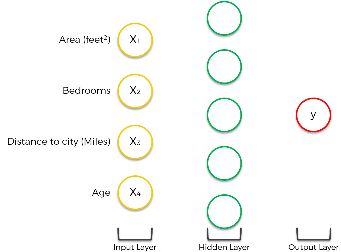
How do hidden layers provide flexibility and functionality? Let’s assume that the first neuron in the hidden layer is affected by area and distance.
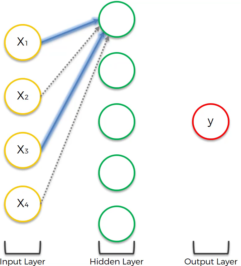
Since all other neurons are also affected in a specific way the result will be:
After that, each neuron in the hidden layer will be calculated by a certain algorithm, similar to the basic form of a neural network.
How do Neural Networks Learn?
To sum up, neural networks learn by adjusting the weights of nodes until the cost $C$ is significantly reduced. The formula for cost $C$ is:
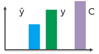
To explain this further, suppose there is a neuron and the actual value $y$ as shown in the image below.
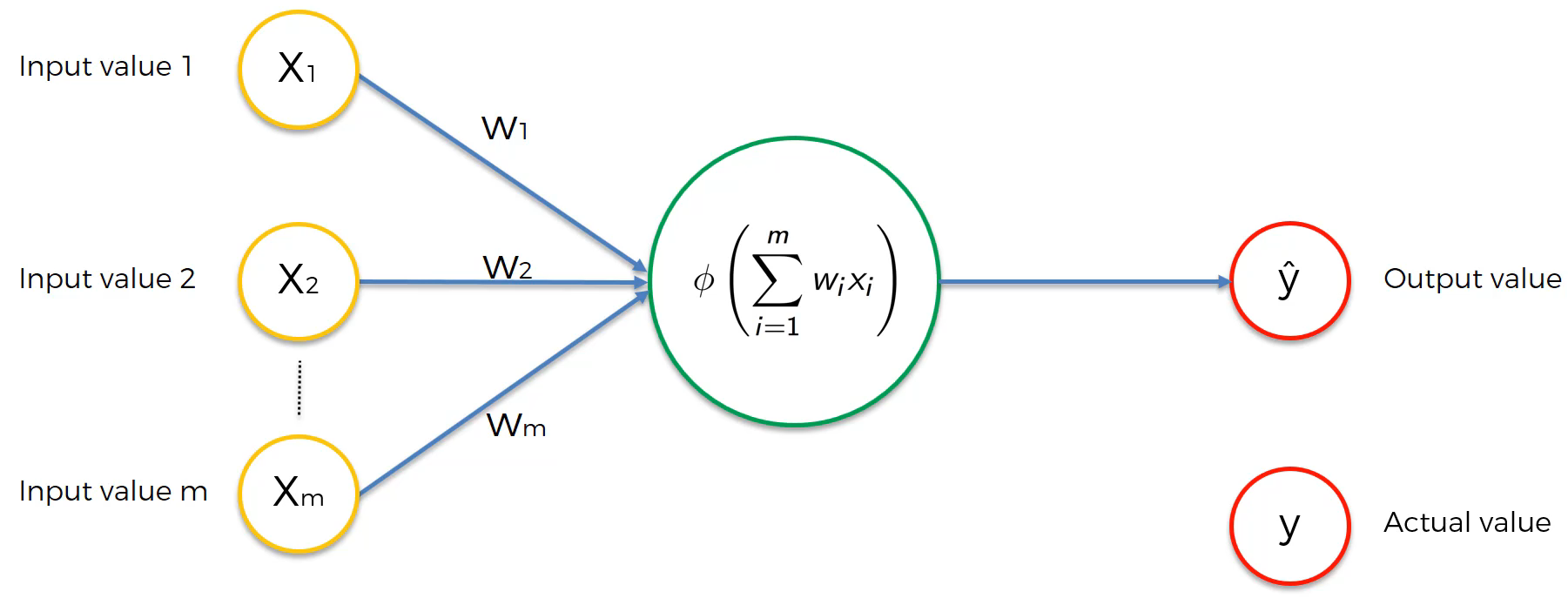
The first activation (forward propagation) through this neuron gives us the predicted value $\hat{y}$ and the cost $C$.
And those values are:
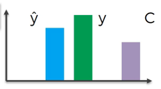
Since the cost $C$ is too high, we backpropagate the information to update the weights.
With the newly updated weights, we activate the neuron again and get the result like:
We repeat the above process until the cost $C$ is significantly low. Although the cost $C$ does not become zero in normal cases, we get:
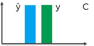
A series of processes that reduce the value of the cost $C$ above is called Gradient Descent.
Example
Code
1
2
3
4
5
6
7
8
9
10
11
12
13
14
15
16
17
18
19
20
21
22
23
from sklearn.preprocessing import StandardScaler
import tensorflow as tf
from sklearn.metrics import confusion_matrix, accuracy_score

sc = StandardScaler()
X_train = sc.fit_transform(X_train)
X_test = sc.transform(X_test)

ann = tf.keras.models.Sequential()
ann.add(tf.keras.layers.Dense(units=6, activation='relu'))
ann.add(tf.keras.layers.Dense(units=6, activation='relu'))
ann.add(tf.keras.layers.Dense(units=1, activation='sigmoid'))

# optimizer='adam' : parameter for stochastic gradient descent
# Loss function used in binary classification: binary_crossentropy
# Loss function used when non-binary classification: categorical_crossentropy
ann.compile(optimizer='adam', loss='binary_crossentropy', metrics=['accuracy'])
ann.fit(X_train, y_train, batch_size=32, epochs=100)
y_pred = ann.predict(X_test)

cm = confusion_matrix(y_test, y_pred)
print(cm)
accuracy_score(y_test, y_pred)
Result
1
0.863