Autoencoder

What is Autoencoder?

An autoencoder is an unsupervised deep learning algorithm used for:

• Feature detection.
  When an autoencoder encodes data, the hidden layer represents important features, which can be used.
• Recommendation systems.
  
• Data encoding.
  

An autoencoder encodes data by taking inputs, passing them through the hidden layer, and then producing outputs with the same number of dimensions as the inputs.

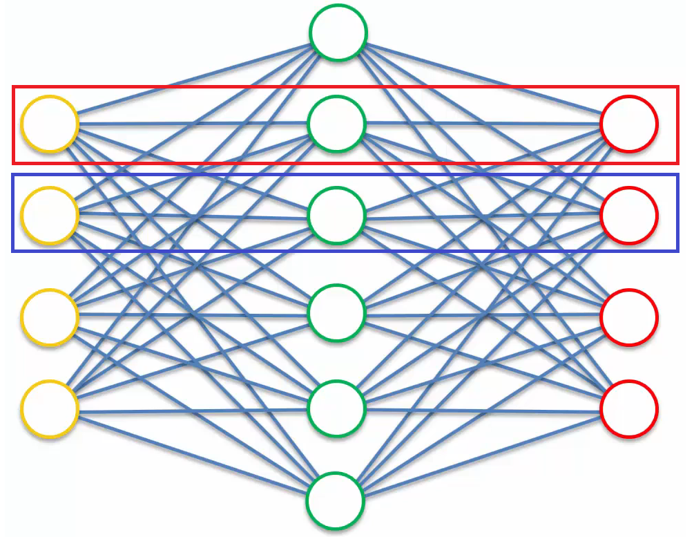
Here is a simple structure of an autoencoder:

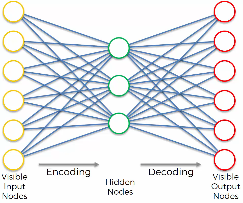
An autoencoder is a directed type of neural network, unlike the boltzmann machine.

How does an Autoencoder Work?

Here is a simplified autoencoder:

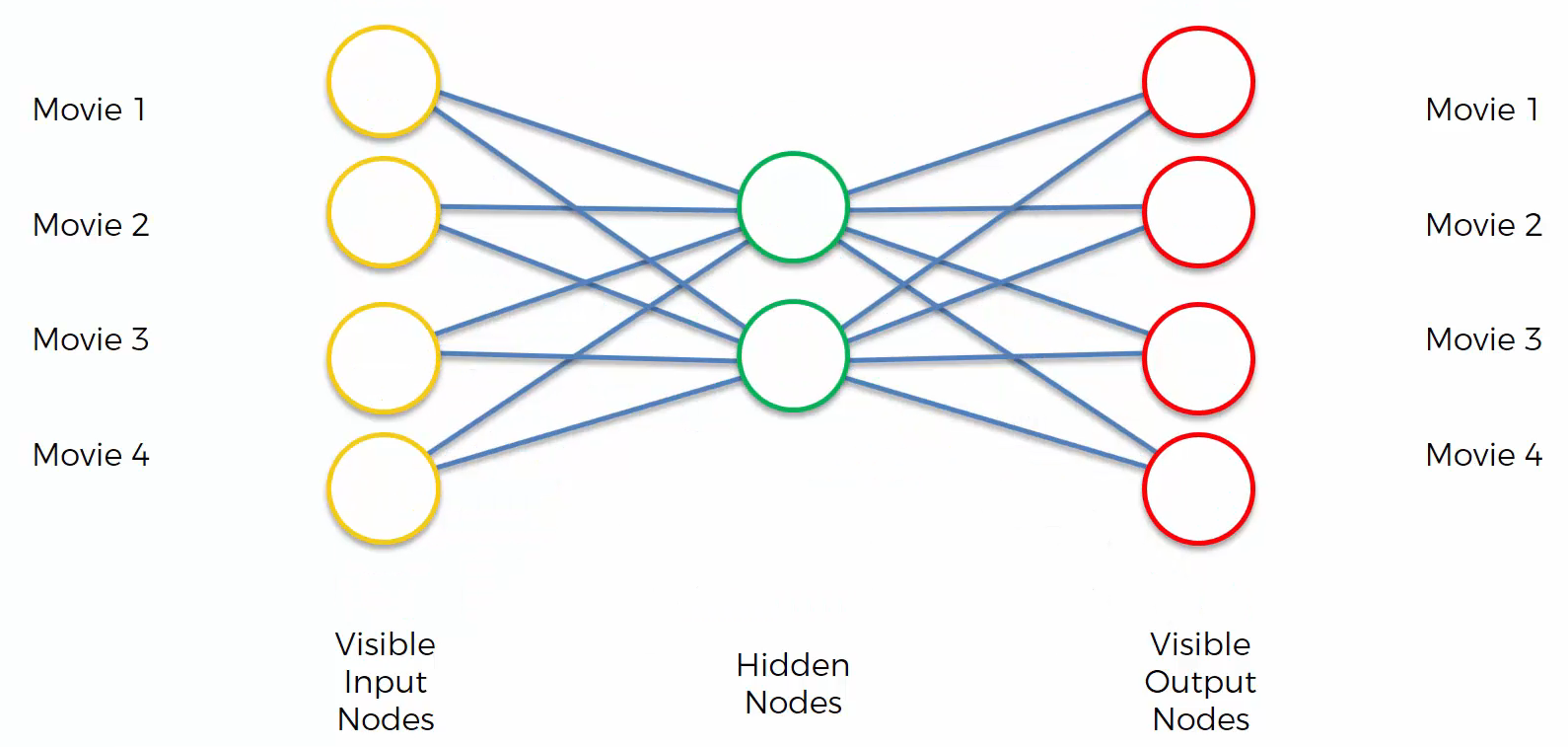
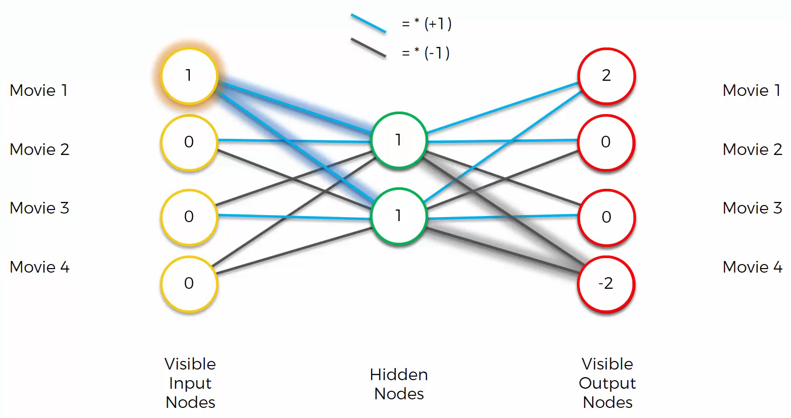
We are going to encode the ratings of movies that people have rated. “1” means they liked the movie and “0” means they didn’t like the movie.
And then, as an example, set the weights like:

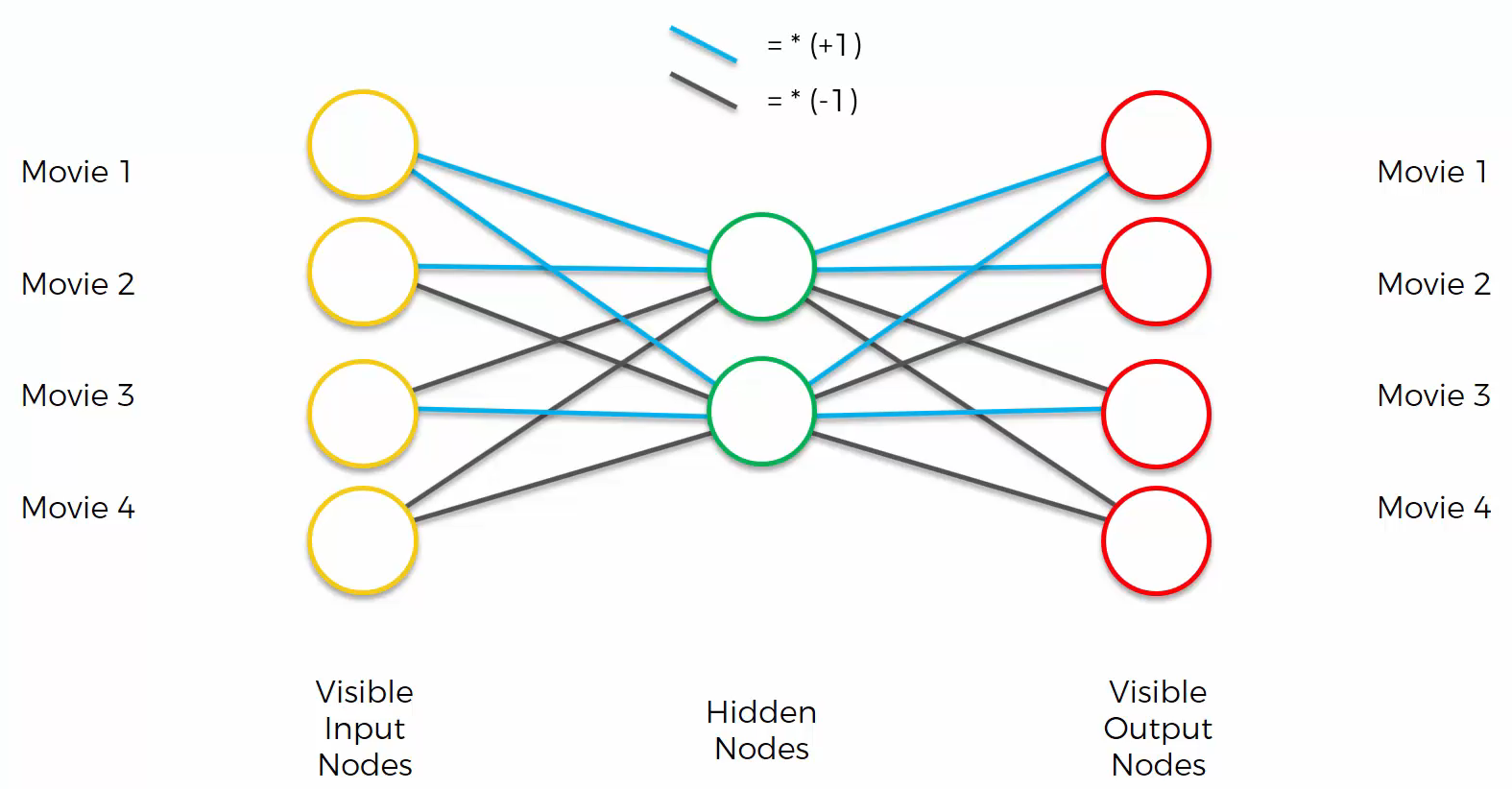
Although we set the weights as shown in the image above as an example, in an autoencoder, the hyperbolic tangent function is usually used to set weights.


We get the input “[1 0 0 0]”.

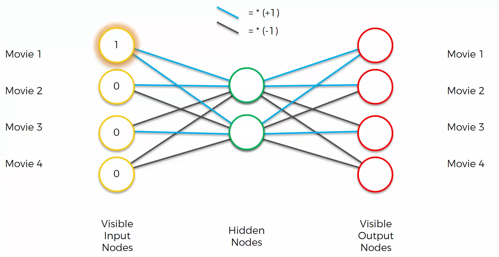
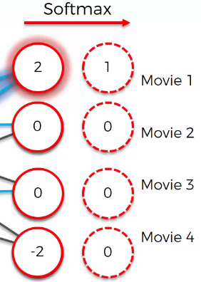
Computing the input with the weights gives the output “[2 0 0 -2]”.

However, this is not the end. By using softmax function, the output becomes “[1 0 0 0]”

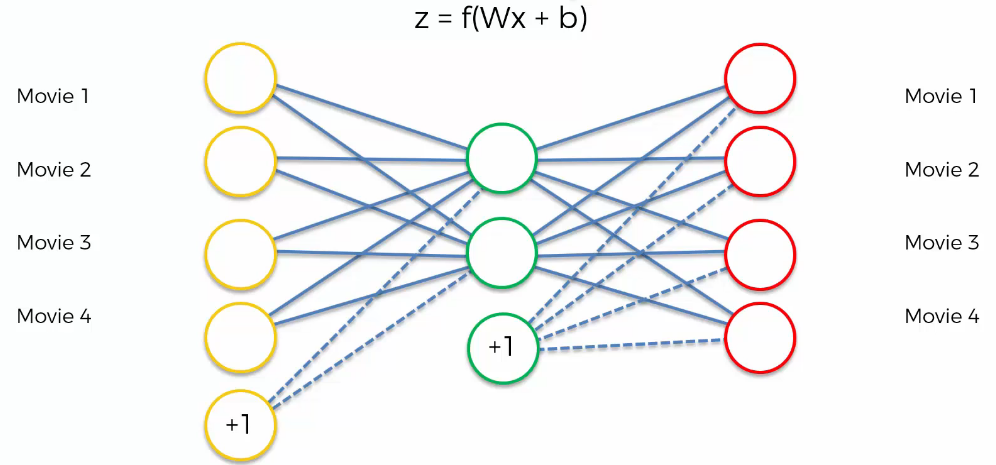
In this case, the input is the same as the output. So, how do you solve the case where the output is not the same as the input? Adding biases is an easy solution.

Training Steps of an Autoencoder

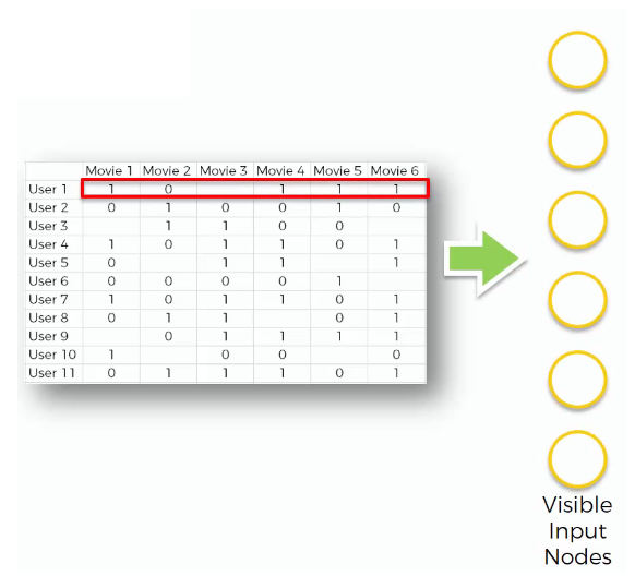
Let’s see the steps of training with an example. As an example, we have movie ratings from various users.

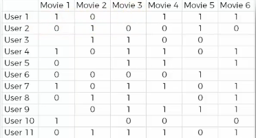
• STEP 1
  We start with an array where the rows (the observations) correspond to the users and the columns (the features) correspond to the movies. Each cell (u, i) contains the rating (from 1 to 5, 0 if no rating) of the movie i by the user u.
  

• STEP 2
  The first user goes into the network. The input vector $x = (r_{1}, r_{2}, \ldots, r_{m})$ contains all its ratings for all the movies.
  

• STEP 3
  The input vector x is encoded into a vector z of lower dimensions by a mapping function f (e.g: sigmoid function):
  

$z = f(Wx + b)$ where W is the vector of input weights and b the bias

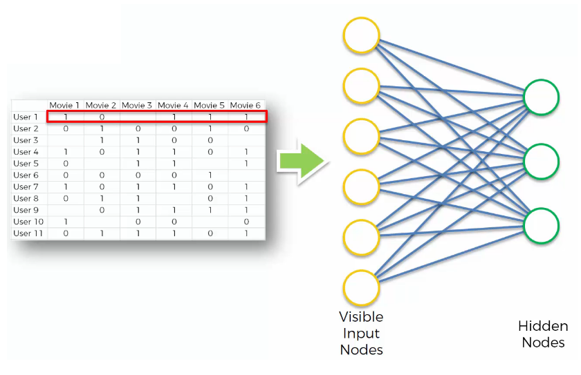
          Although there is randomly initialized weights, encoding is performed.

• STEP 4
  z is then decoded into the output vector y of same dimensions as x, aiming to replicate the input vector x.
  

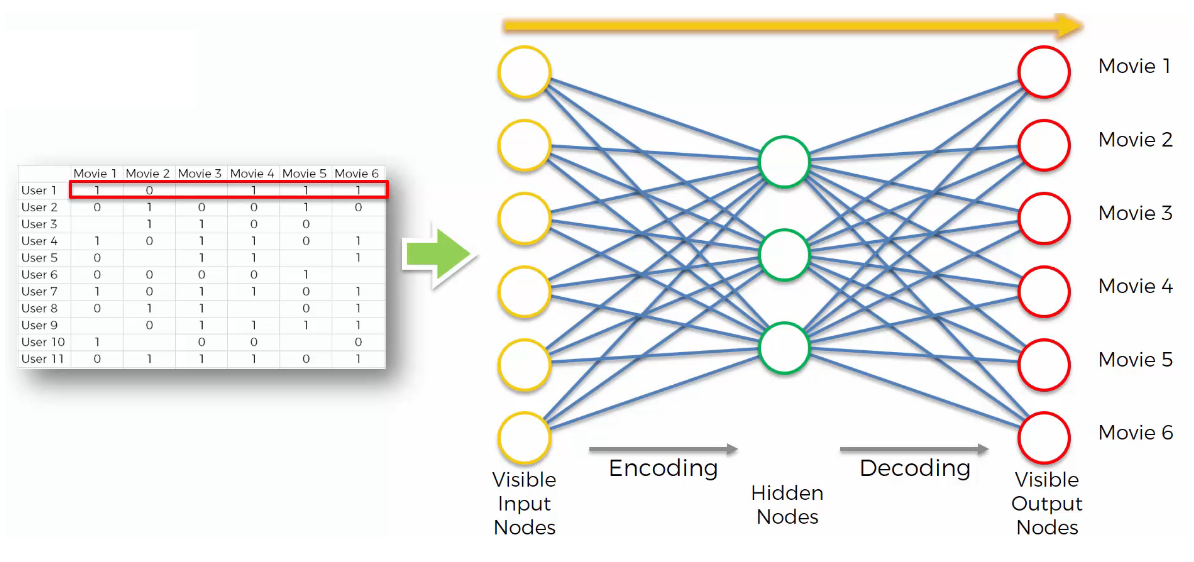
• STEP 5
  The reconstruction error d(x, y) = $||x\ -\ y||$ is computed. The goal is to minimize it.
  
• STEP 6
  Back-Propagation: from right to left, the error is back-propagated. The weights are updated according to how much they are responsible for the error. The learning rate decides by how much we update the weights.
  

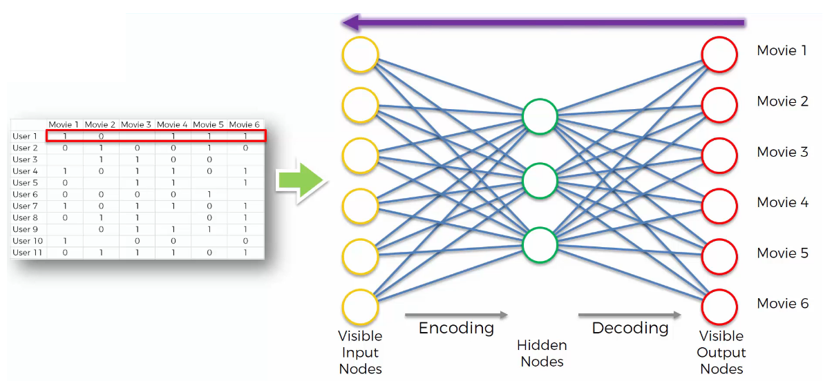
• STEP 7
  Repeat Steps 1 to 6 and update the weights after each observation (Reinforcement Learning).
  Or Repeat Steps 1 to 6 but update the weights only after a batch of observations (Batch Learning).
  

• STEP 8
  When the whole training set passed through the ANN, that makes an epoch. Redo more epochs.
  
  
  
  

Overcomplete Hidden Layers

Overcomplete hidden layers are used in many variations of autoencoders. For example, if we want to use an autoencoder as a feature extractor and get more features by having more hidden nodes than input nodes, we can use overcomplete hidden layers.
However, there is a problem. If there are more hidden nodes than input nodes, the autoencoder can use a “cheat” like “values in boxes of the same color are always the same.”

In this way, we can’t extract any valuable features from the autoencoder. To solve this problem, there are several different types of autoencoders, which I’ll introduce below.

Types of Autoencoders

• Sparse Autoencoder
  

• Denoising Autoencoder
  

• Contractive Autoencoder
  

• Stacked Autoencoder
  

• Deep Autoencoder
  

Example

Code

import numpy as np
import pandas as pd
import torch
import torch.nn as nn
import torch.nn.parallel
import torch.optim as optim
import torch.utils.data
from torch.autograd import Variable

# Importing the data
movies = pd.read_csv('ml-1m/movies.dat', sep='::', header=None, engine='python', encoding='latin-1')
users = pd.read_csv('ml-1m/users.dat', sep='::', header=None, engine='python')
ratings = pd.read_csv('ml-1m/ratings.dat', sep='::', header=None, engine='python')

# Preparing the training set and the test set
training_set = pd.read_csv('ml-100k/u1.base', delimiter='\t', )
training_set = np.array(training_set, dtype='int')
test_set = pd.read_csv('ml-100k/u1.test', delimiter='\t', )
test_set = np.array(test_set, dtype='int')


# Getting the number of users and movies
nb_users = max(max(training_set[:, 0]), max(test_set[:, 0]))
nb_movies = max(max(training_set[:, 1]), max(test_set[:, 1]))

# Converting the data into an array with users in lines and movies in columns
def convert(data):
    new_data = []
    for id_users in range(1, nb_users + 1):
        id_movies = data[:, 1][data[:, 0] == id_users]
        id_ratings = data[:, 2][data[:, 0] == id_users]
        ratings = np.zeros(nb_movies)
        ratings[id_movies - 1] = id_ratings
        new_data.append(list(ratings))
    return new_data
training_set = convert(training_set)
test_set = convert(test_set)

# Converting the data into Torch tensors
training_set = torch.FloatTensor(training_set)
test_set = torch.FloatTensor(test_set)


# Creating the architecture of the Neural Network
class SAE(nn.Module):
    def __init__(self,):
        super(SAE, self).__init__()
        # Full connection connected to autoencoder
        # Linear (input vector, number of hidden neurons)
        self.fc1 = nn.Linear(nb_movies, 20)
        self.fc2 = nn.Linear(20, 10)
        """Since no more encoding layers are added, the number of hidden neurons is configured equal to the number of input vectors at the beginning.
            = decoding"""
        self.fc3 = nn.Linear(10, 20)
        self.fc4 = nn.Linear(20, nb_movies)
        self.activation = nn.Sigmoid()
        
    # Define action in autoencoder
    def forward(self, x):
        x = self.activation(self.fc1(x))
        x = self.activation(self.fc2(x))
        x = self.activation(self.fc3(x))
        x = self.fc4(x)
        return x
    
sae = SAE()
criterion = nn.MSELoss()
optimizer = optim.RMSprop(sae.parameters(), lr=0.01, weight_decay=0.5)

# Training the SAE
epochs = 200
for epoch in range(1, epochs+1):
    train_loss = 0
    s = 0.
    for id_user in range(nb_users):
        input = Variable(training_set[id_user]).unsqueeze(0)
        target = input.clone()
        if torch.sum(target.data > 0) > 0:
            output = sae(input)
            # Calculate descent
            target.require_grad = False
            output[target == 0] = 0
            loss = criterion(output, target)
            # Average the ratings of the rated movies
            mean_corrector = nb_movies/float(torch.sum(target.data > 0) + 1e-10)
            loss.backward()
            train_loss += np.sqrt(loss.data*mean_corrector)
            s += 1.
            optimizer.step()
            """Difference between backward and step
               backward : direction
               step: mass"""
    print('epoch:', epoch, 'loss:', (train_loss/s))
    
# Testing the SAE
test_loss = 0
s = 0.
for id_user in range(nb_users):
    # The reason for leaving the input as training set: Because the items predicted in the training set are in the test set and can be compared together
    input = Variable(training_set[id_user]).unsqueeze(0)
    target = Variable(test_set[id_user]).unsqueeze(0)
    if torch.sum(target.data > 0) > 0:
        output = sae(input)
        target.require_grad = False
        output[target == 0] = 0
        loss = criterion(output, target)
        mean_corrector = nb_movies/float(torch.sum(target.data > 0) + 1e-10)
        loss.backward()
        test_loss += np.sqrt(loss.data*mean_corrector)
        s+=1.
        optimizer.step()
    print('loss:', (test_loss/s))

Result

Implementation

• AutoEncoder 1
  
• AutoEncoder 2
  
• Classify autoencoded images by CNN