Long Short-Term Memory Networks(LSTM)

What is LSTM?

LSTM is devised to solve the vanishing gradient problem in RNN. Here is a basic structural image of LSTM:

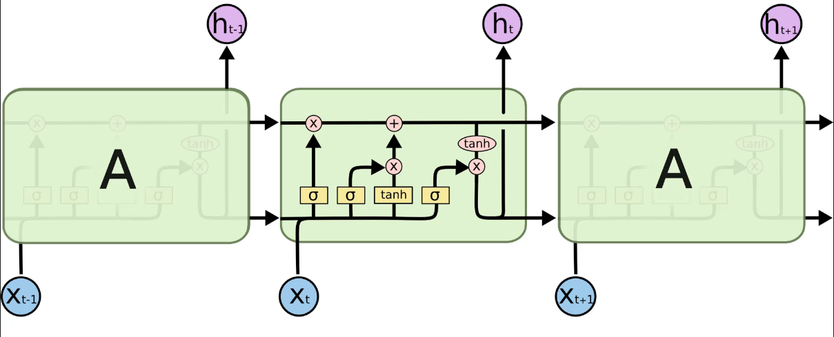
The meanings of the symbols are shown below:

One thing to notice is that $W_{rec}$ is fixed at 1. In LSTM, the top side pipeline, called the memory cell, represents $W_{rec}$.

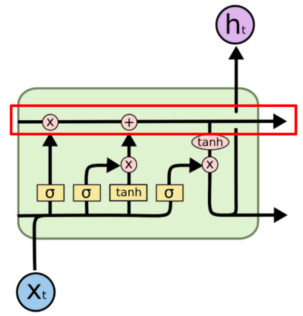
In the memory cell, information can freely flow through time. Sometimes it might be erased in the $\times$ circle or added in the $+$ circle.
To make it easier to understand, let’s assume that we are translating. In the cell, the information about a boy goes through.

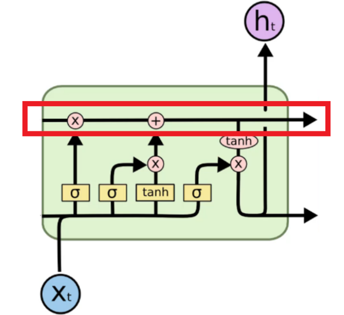
The information about the boy goes through until there is a new input in $X_{t}$. So, let’s assume ‘girl’ is entered as a new input in $X_{t}$.

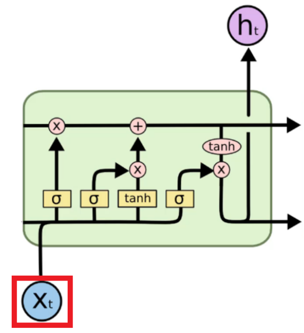
Then, LSTM orders open and close some “pointwise operations”.

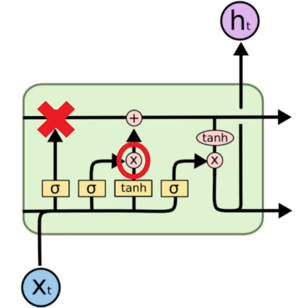
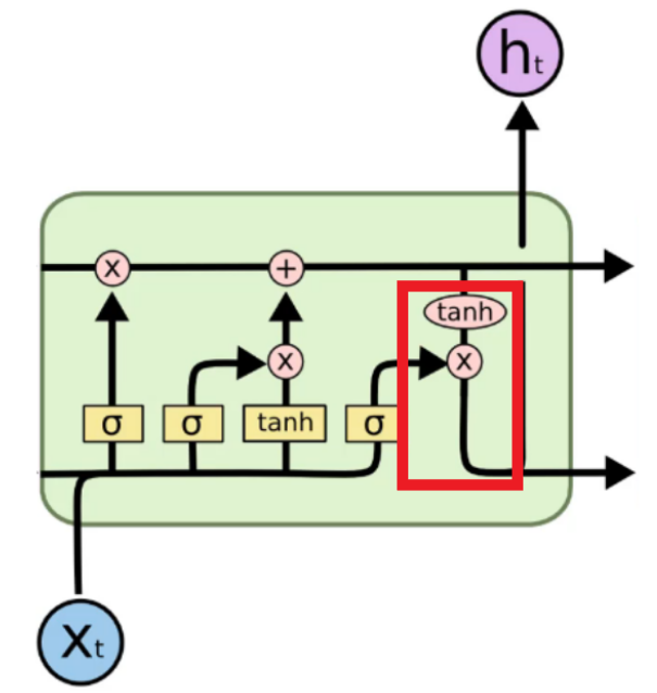
By doing this, the memory for the boy is erased, and we have a new memory for the girl. In the cell, certain information is extracted, and this information will be the input for the next cell.

Variants of LSTM

---

• Adding peephole connections
  It adds some lines to provide additional information about the current state of the memory cell to the sigmoid activation function layers.

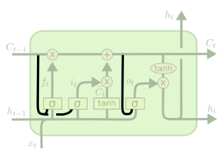
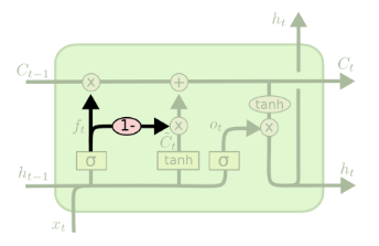
• Use coupled forget and input gates
  These gates interact so that when one is 1, the other is 0. In other words, nothing is added to the memory cell, keeping the value of the memory cell constant.

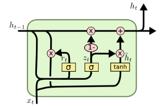
• Gated Recurrent Unit (GRU)
  There is no memory cell; instead, it is replaced by a hidden pipeline.

Example

Code

---

from sklearn.preprocessing import MinMaxScaler
from keras.models import Sequential
from keras.layers import Dense
from keras.layers import LSTM
from keras.layers import Dropout

sc = MinMaxScaler(feature_range=(0, 1))
training_set_scaled = sc.fit_transform(training_set)
""" number of timesteps : 
    A data structure that specifies what the RNN should remember when predicting the next stock price.
    n timestep: last ~ last - n data
     """
X_train = []
y_train = []
for i in range(60, len(training_set)):
    X_train.append(training_set_scaled[i-60 : i, 0])
    y_train.append(training_set_scaled[i, 0])

X_train, y_train = np.array(X_train), np.array(y_train)

X_train = np.reshape(X_train, (X_train.shape[0], X_train.shape[1], 1))

regressor = Sequential() # Regression is used because it predicts continuous values.
"""units : the number of neurons the LSTM will have in each layer
   return_sequence: When adding another layer after the LSTM layer: true / false if not added
   input _hape : timesteps(X_train.shape[1])
   rate: The number of neurons to drop per layer"""
regressor.add(LSTM(units=50, return_sequences=True, input_shape=(X_train.shape[1], 1)))
regressor.add(Dropout(rate=0.2))
# Reason for not specifying input_shape : Because input_shape is provided in the first LSTM layer
regressor.add(LSTM(units=50, return_sequences=True)) 
regressor.add(Dropout(rate=0.2))
regressor.add(LSTM(units=50, return_sequences=True))
regressor.add(Dropout(rate=0.2))
regressor.add(LSTM(units=50))
regressor.add(Dropout(rate=0.2))
regressor.add(Dense(units=1))
regressor.compile(optimizer='adam', loss='mean_squared_error')

regressor.fit(X_train, y_train, epochs=100, batch_size=32)

predicted_stock_price = regressor.predict(X_test)

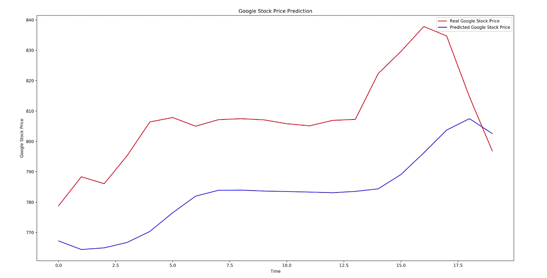
Result

---

Implementation

• LSTM 1
• LSTM 2
• LSTM 3